mueller
The Redacted Mueller Report
Who has time to read through over 400 pages to find out what is in the Mueller Report? Not Me! So when I found the link to the pdf version of the report I wondered what type of stuff was in there and sought out to extract some meaning from the report. This was my motivation when starting this project.
Project Overview
The goal of this project is to analyze the Mueller Report with visualizations and Sentiment Analysis.
Data Processing and Cleaning
Data downloaded from CNN as a PDF report and there were 448 pages in the report.
To get the data in a usable format, the PDF report had to be converted to text format:
def parsePDF(filename, page_start, page_end):
    '''

    :param filename: PDF file to extract data from
    :param page_start: integer - start page
    :param page_end: integer - end page
    :return: string with text
    '''
    # name of PDF file to parse (creates an object)
    pdfFileObj = open(filename,'rb')
    # pdfReader will be parsed
    pdfReader = PyPDF2.PdfFileReader(pdfFileObj)
    # get start and end pages
    if not page_start:
        start = 1
    else:
        start = page_start
    if not page_end:
        end = pdfReader.numPages
    else:
        end = page_end

    # go through each page and extract text to string
    text = ''
    for i in range(start, end):
        print("processed page" , str(i))
        pageObj = pdfReader.getPage(i)
        text += pageObj.extractText()
    return(text)
Once the data was extracted using pdfReader in Python, data cleaning involved removing digits, punctuation and converting all words to lowercase. Stopwords such as “the”, “and”, “as”, “of” were also removed by using the NLTK libary and words were returned to root form using lemmatization. I used lemmatization over stemming because I wanted the data to include actual words and stemming sometimes can return words that aren’t in fact real words. There are cases where stemming is helpful in data pre-processing but in my case this wouldn’t have helped me understand which words were used most frequently.
Lemmatization with Python nltk package: “Lemmatization, unlike Stemming, reduces the inflected words properly ensuring that the root word belongs to the language. In Lemmatization root word is called Lemma. A lemma (plural lemmas or lemmata) is the canonical form, dictionary form, or citation form of a set of words.”
def get_tokens(text_string):
    '''
    Function that takes in text string and returns list of words
    removes stop words & empty spaces & words with less then 2 characters

    :param text_string: text string
    :return: list of words
    '''
    from nltk.tokenize import word_tokenize
    from nltk.corpus import stopwords as stopWords

    stop_words = set(stopWords.words('English'))
    # split words into list
    tokens = word_tokenize(text_string)

    # remove stop words
    tokens = [word for word in tokens if word not in set(stopWords.words("English"))]
    tokens = [word for word in tokens if word not in stop_words]
    tokens = [word for word in tokens if word != '']
    tokens = [word for word in tokens if len(word) > 2]
    return tokens

def lematize_word(word):
    '''
    Function to return lemma for a word - uses WordNetLemmatizer
    1) find part of speech tag (pos)
    2) convert penn tag to wordnet tag
    3) return lemma based on tag

    :param word: string to lemmatize
    :return: lemma (str)
    '''
    from nltk.stem import WordNetLemmatizer
    from nltk import pos_tag
    if word == '':
        pass
    res = pos_tag([word])

    word, pos = res[0][0], res[0][1]
    # convert to wordnet tag
    tag = penn_to_wn(pos)
    if tag:
        wnl = WordNetLemmatizer()
        token_lem = wnl.lemmatize(word, pos=tag)
        return token_lem
    else:
        pass

# lematize words
lemmas = [lematize_word(x) for x in cleaned_words if x]
lemma_counts = Counter(lemmas)
print("top 10 words found in report", lemma_counts.most_common(20))
Data Exploration & Visualization
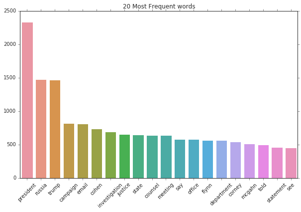
Now that the data is cleaned, we can move on to some visualization… what words appear the most? Not surprisignly, “president”, “Russia”, “Trump”, “campaign”, “investigation” appear very frequently in the report:
WordClouds
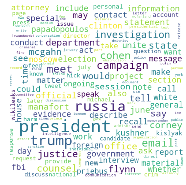
A pretty neat way of visualizing words is by creating wordclouds, which is quite straightforward and simple using the wordcloud library:
# put words and frequencies in a dataframe
df_wordcounts = pd.DataFrame(list(lemma_counts.most_common(21)), columns=['words','freq'])

wordcloud = WordCloud(width = 512, height = 512, background_color='white', max_font_size=50, max_words=150)
wordcloud = wordcloud.generate_from_frequencies(df_wordcounts.set_index('words').freq)
plt.figure(figsize=(10,8),facecolor = 'white', edgecolor='blue')
plt.imshow(wordcloud, interpolation="bilinear")
plt.axis("off")
plt.tight_layout(pad=0)
plt.show()
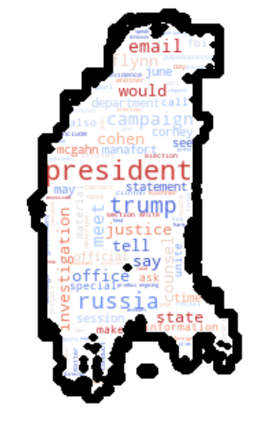
We could also make a wordcloud in a specific shape based on a picture, for example:
from matplotlib import cm
# generate wordcloud with custom settings
wordcloud = WordCloud(width = 512, height = 512, background_color='white', colormap=cm.coolwarm, contour_width=10, contour_color='black', max_font_size=70, max_words=150)
mueller_mask = np.array(Image.open("img/mask2.jpeg"))
# change the shape of the wordcloud
wordcloud.mask = mueller_mask
# generate from frequencies
wordcloud = wordcloud.generate_from_frequencies(df_wordcounts.set_index('words').freq)

# show plot
plt.figure(figsize=(10,8),facecolor = 'white', edgecolor='blue')
plt.imshow(wordcloud, interpolation="bilinear")
plt.axis("off")
plt.tight_layout(pad=0)
plt.show()
But… Is this a bird or a dinosaur wordcloud?
Sentiment Analysis
In this section the text data that was converted from pdf to text sentences was parsed, cleaned and each word was tagged with a part of speech. Stopwords, words with fewer than 3 characters are removed so that we can focus on words with meaning in the data.
Data Part of Speech Tagging and Sentiment Scoring:
To find out whether a word is positive or negative, I used SentiWordNet from NLTK library to compute sentiment polarity scores. From NLTK: “SentiWordNet is a lexical resource for opinion mining and it assigns to each synset of WordNet three sentiment scores: positivity, negativity and objectivity.”
The SentiWordNet functionality provides the synsets function to convert a word and part of speech tag to a filter object with a positive, negative and objective score.
A few additional steps have to be taken in order to be able calculate the sentiment score:
- convert from Penn Treebank part of speech tag to WordNet part of speech tag (this is done using the penn_to_wn function)
- lemmatize words based on simple WordNet tag
- convert lemma to synsets filter object and pick the most common synset from list (this is the 1st item)
- finally subtract the negative score from the positive score
def get_swn_word_sentiment(token, tag):
    """
        Function to retrieve sentiment polarity average between negative, positive sentiment based on SentiWordNet
        Objective sentiment is not included in sentiment score
        Sentiment score = positive - negative score

        Input: str
        Output: float
    """
    senti_score = 0.0
    lemmatizer = WordNetLemmatizer()
    # convert to WordNet part of speech tag
    wn_tag = penn_to_wn(tag = tag)

    # other tags arent supported by sentiword
    if wn_tag not in (wn.NOUN, wn.ADJ, wn.ADV, wn.VERB):
        pass
    else:
        lemma = lemmatizer.lemmatize(token, wn_tag)

        if not lemma:
            pass
        else:
            try:
                # convert word to synset
                synsets = swn.senti_synsets(lemma, pos = wn_tag)
                if not synsets:
                    pass
                else:
                    synset = synsets[0]
                    # return positive - negative sentiment score
                    senti_score = synset.pos_score() -  synset.neg_score()
                    return senti_score
            except:
                pass
The input for the above function is a word and its Penn Treebank tag, so the only thing remaining to do is to loop through our sentences and get the part of speech tag for each word in each sentence and word sentiment. In the below I only keep words where the sentiment score is above 0:
'''
    loop through sentences and get sentiment score for each word
    ignore words where sentiment = 0
    keep track of results in 4 lists: important words, sentiment scores, part of speech tags, and sentence index position
'''

# create a list for each sentence
sentences = sent_tokenize(text_result)

imp_words = []
scores = []
tags = []
ids = []

for ix, sentence in enumerate(sentences):
    for word, tag in pos_tag(get_tokens(sentence)):
        lemmatizer = WordNetLemmatizer()
        word_sentiment = get_swn_word_sentiment(word, tag)
        if word_sentiment > 0:
            lemma = lemmatizer.lemmatize(word, penn_to_wn(tag))
            print("word: {}, lemma: {}, tag: {}, sentiment: {}".format(word, lemma, tag, word_sentiment))
            imp_words.append(lemma)
            scores.append(word_sentiment)
            tags.append(tag)
            ids.append(ix)
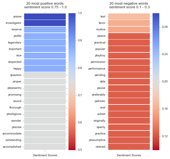
Sorting the results by words with highest sentiment scores, it looks like most of these were correctly given positive scores. We can see words such as nice, happy and praise at the top of the list:
| imp_words | score_counts | score_mean |
|---|---|---|
| investigator | 44 | 1 |
| praise | 2 | 1 |
| important | 35 | 0.875 |
| happy | 6 | 0.875 |
| prefer | 2 | 0.875 |
| respected | 2 | 0.875 |
| legendary | 1 | 0.875 |
| nice | 1 | 0.875 |
| reserve | 1 | 0.875 |
| constitutional | 73 | 0.75 |
| emphasis | 12 | 0.75 |
| question | 11 | 0.75 |
| proper | 7 | 0.75 |
| wonderful | 5 | 0.75 |
| competent | 2 | 0.75 |
| favorable | 2 | 0.75 |
| outstanding | 2 | 0.75 |
| wonder | 2 | 0.75 |
| accommodate | 1 | 0.75 |
| accomplished | 1 | 0.75 |
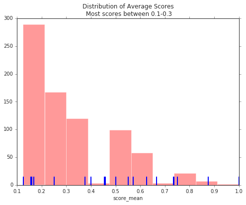
Plotting the distribution of our scores, most words are negative in the report with scores between 0.1 and 0.3:
# plot distribution of scores
fig, ax = plt.subplots(figsize = (8,6))
_ = sns.distplot(word_stats.score_mean, bins = 10, ax = ax, rug=True, hist=True, kde=False,
             hist_kws={'color':'red','stacked':True},
             rug_kws={'color':'blue','lw':2} )
ax.set_title('Distribution of Average Scores\n Most scores between 0.1-0.3')
plt.show(fig)
Heatmaps of Most Positive and Negative Words in Report
The most positive words are plotted on the left with ‘praise’, ‘happy’, ‘pleasantry’ and ‘respected’ scoring high above 0.7. Negative words such as ‘noticed’, ‘presumptive’,’playboy’, ‘patriotic’, and’question’ have the lowest sentiment scores below 0.2:
