Facebook Promoted Posts
This repository includes a jupyter notebook which implements machine learning models such as logistic regression, decision trees and random forests using sci-kit learn to predict whether a Facebook post is promoted or not. The problem is a classification problem, where I created the labels for promoted or not based on impressions paid.
Project Motivation
Facebook has many pages and posts that people look at on a daily basis. While many of us may not pay attention to the sponsored posts, there are quite a lot of these paid posts that take up space on our Facebook feeds. But how can you tell if a post is paid without looking for the Sponsored label? Do these paid posts have higher number of views just because they are paid for? The question I wanted to answer was: can we predict if a Facebook post is promoted or not?
Data Collection
In order to get the data I was looking for, I used the below SQL query on a sqlite database which contained facebook pages, posts and posts-insights data. I used an inner join to join the pages and posts tables to get access to page information such as facebook page id from the pages table and facebook post id from the posts table. I added another inner join to join post with post-insights data to have access to post insights fields such as impressions paid, organic impressions, post consumption by type, post video views. Since the goal of this project was to predict if a post was promoted or not, I defined a post as promoted when there were more than 0 impressions paid for that post, and otherwise I labeled the post as not promoted. This is the response variable that I was aiming to predict.
select p.id, p.facebook_page_id, p.name, po.page_id, po.facebook_post_id,
ps.impressions_paid_unique, ps.impressions_fan_paid_unique, ps.impressions_fan_unique, ps.impressions_organic_unique,
ps.impressions_by_story_type_unique_other,
ps.consumptions_by_type_unique_link_clicks, ps.consumptions_by_type_unique_photo_view, ps.consumptions_by_type_unique_video_play,
ps.consumptions_by_type_unique_other_clicks, ps.consumptions_unique,
ps.negative_feedback_by_type_unique_hide_clicks, ps.negative_feedback_by_type_unique_hide_all_clicks, ps.negative_feedback_unique,
ps.video_views_paid_unique, ps.video_views_organic_unique, ps.video_complete_views_organic_unique, ps.video_complete_views_paid_unique,
CASE
WHEN ps.impressions_paid_unique > 0 THEN 1
ELSE 0
END as is_promoted
from pages as p
inner join posts as po on p.id = po.page_id
inner join post_insights as ps on ps.post_id = po.id
Data Cleaning
To clean the data, I created a little helper function to take care of some of the following processing tasks: removing columns where more than 80% of the data was missing, filling in missing values based on the average for that facebook page id and fixing column names. My thoughts were that if a column has more than 80% of its values missing, then there is not much information in that column and it should be removed. What can we learn from an empty column after all? The clean function also changed facebook page names to lower letters and converted facebook page ids to string type. I included the option to remove columns where there was paid information, in case I would want to remove these columns later.
'''
Fill in NA values
1) using average for that group for that column
2) using average of that column (this only happens if there s still NAs)
3) option to delete columns with "paid"
'''
def clean(dat, threshold = 0.80, delete_paid = False):
    dat = dat.copy()

    dat.drop([c for c in dat if dat[c].isnull().sum()/nrows >.80], axis = 1, inplace=True)
    if delete_paid:
        dat.drop([x for x in dat.columns if 'paid' in x], axis = 1, inplace = True)
    dat.facebook_page_id = dat.facebook_page_id.astype(np.str)
    dat.name = dat.name.map(lambda x: x.lower())

    cols_fill = [c for c in dat.columns if (dat[c].isnull().sum()/nrows < threshold) and (dat[c].isnull().sum()/nrows >0.00)]
    for i in cols_fill:
        dat[i].fillna(dat.groupby('facebook_post_id')[i].transform("mean"), inplace = True)
        dat[i].fillna(dat[i].mean(), inplace = True)
    return dat
Data Exploration
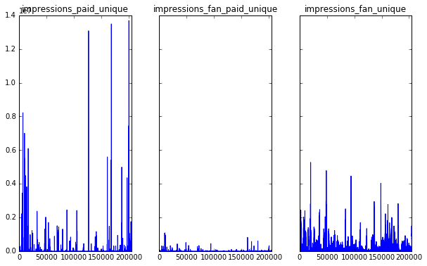
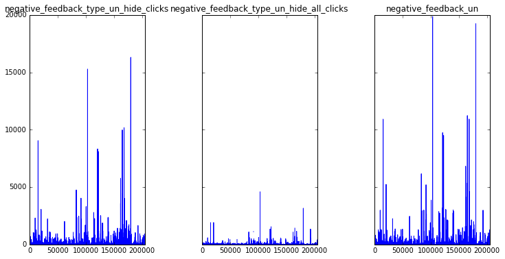
After quickly plotting the features, I noticed that impressions fan unique, consumptions unique, negative feedback unique and video views organic unique seemed to have a widder range of values, and perhaps higher variance than the other features that had more zero values.
sub_dat = df_joined.ix[:, 19:22]
fig, axes = pyplot.subplots(nrows=1, ncols=3, figsize=(12,6), sharey=True)
for i, var in enumerate(sub_dat.columns):
    l = var.replace('consumptions', 'cons').replace('impressions','imp').replace('by_','').replace('unique','un')
    sub_dat[[i]].plot(ax = axes[i], title = l, legend ='')
fig.subplots_adjust(hspace=0.5, wspace=0.5)
pyplot.show()


Machine Learning Algorithms - Logistic Regression and Decision Tree Classifier
Since this is a classification problem where we predict if a post is promoted (let’s call this class 1) or not promoted (class 0, I chose to use Logistic Regression and Decision Tree classifiers. Both of these are simple supervised machine learning classification algorithms that can be implemented quickly and are pretty interpretable.
1 - Logistic Regression on entire dataset
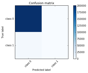
I started off by trying logistic regression on the entire data and was not shocked to see that it performed poorly by predicting all posts as not promoted (class 0). Since most of the posts in the dataset are not promoted, this is not surprising. The accuracy score is high, which means that the model predicted many of the points correctly. While accuracy is a measure of how well the model performed, the fact that the accuracy score is high does not indicate that this is a good model.
The model correctly predicted all of the non-promoted posts correctly, but it missed the promoted posts and predicted all of these as non-promoted also. Looking at the confusion matrix, we see that none of the points in the positive class (promoted) were correctly predicted.
cols_train = data.drop('is_promoted', axis = 1).columns
X = data[cols_train]
y = data.is_promoted
target_names = ['class 0', 'class 1']

logreg = LogisticRegression(C=1e9)
logreg.fit(X,y)
data['promo_pred_1'] = logreg.predict(X)
Here we can see that the logistic regression model predicted all posts as non-promoted: Class 0: 204804
The below confusion matrics shows that there were 201448 non promoted posts correctly predicted, while all of the 3356 promoted posts were incorrectly labeled as non-promoted.
Confustion Matrix:
| Non-Promoted Predicted | Promoted Predicted | |
|---|---|---|
| Non-Promoted-Actual | 201448 | 0 |
| Promoted-Actual | 3356 | 0 |
The classification report breaks down the true positive and false positive rates to give better insights into where the model scored well or not. We can see that the promoted posts scored 0 precision and 0 recall, indicating a poor performance.
Classification Report:
| Class | Precision | Recall | F1-Score |
|---|---|---|---|
| Non-Promoted | 0.98 | 1.00 | 0.99 |
| Promoted | 0.00 | 0.00 | 0.00 |
| avg/total | 0.97 | 0.98 | 0.98 |
From the visualization below, it is clear that all posts were predicted as non-promoted:

2 - Logistic Regression on a few features
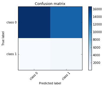
Before performing feature selection, I wanted to try using Logistic Regression and training the model on a few features that I thought would be predictive. I chose impressions fan unique, consumptions unique, negative feedback unique, video views organic unique and impressions organic unique. The accuracy was lower because it was at at 56% but the model predicted some posts to be promoted, so the predictions are a bit more balanced. The precision is low for promoted posts as it incorrectly classifies alot of posts as promoted (false positives). Recall/Sensitivity is low for unpromoted posts - number of prediction unpromoted posts is low in comparison to the total number of unpromoted posts. When looking at coefficients, these seems to indicate some relationship to output, so I needed to work on selecting better features.
'''
Logistic Regression #2 - on .90 dataset & only a few features
'''

X = data[['impressions_fan_unique','consumptions_unique','negative_feedback_unique','video_views_organic_unique','impressions_organic_unique']]
y = data.is_promoted
# training and testing
X_train, X_test, y_train, y_test = cross_validation.train_test_split(X, y, test_size=0.15, random_state=1)
Cs = np.logspace(-4, 4, 3)
logreg3 = LogisticRegression(C=Cs[2], class_weight='balanced', multi_class = 'ovr')
logreg3.fit(X_train,y_train)
promo_pred_3 = logreg3.predict(X_test)
Average accuracy: 55.82%
Model Predictions:
- Class 0: 16829
- Class 1: 13892
Confustion Matrix:
| Non-Promoted Predicted | Promoted Predicted | |
|---|---|---|
| Non-Promoted-Actual | 16744 | 13489 |
| Promoted-Actual | 85 | 403 |

3 - Decision Tree Classifier and feature importance
Below I trained a decision tree classifier on all the features, and it showed that the top 3 features with the most imformation gain were: impressions fan unique, impressions organic unique ,impressions by story type unique other. So, my thoughts on which features could be good predictors were not quite correct. It looks like impressions are very important in predicting whether a post is promoted or not. The model performed alot better than logistic regression. It scored perfectly on unpromoted posts and very well on promoted posts.
'''
FEATURE IMPORTANCE USING DECISION TREE
'''
X, y = shuffle(data.ix[:, 1:-3], data.is_promoted, random_state=23)
X_train, X_test, y_train, y_test = cross_validation.train_test_split(X, y, test_size=0.15, random_state=1)

tree_model = tree.DecisionTreeClassifier(criterion='gini')
tree_model = tree.DecisionTreeClassifier()
tree_model.fit(X_train, y_train)

tree_predicted = tree_model.predict(X_test)
Decision trees select the best feaures to split on at each node and based on the feature with the highest information gain it splits, and they can return the feature importance:
tree_impt = tree_model.feature_importances_

# get sorted index
sorted_idx_tree = np.argsort(tree_impt)
for f in xrange(len(X.columns),0,-1):
    print("%d. feature %d (%f)  %s" % (f , sorted_idx[f-1], tree_impt[sorted_idx_tree[f-1]], X.columns[sorted_idx_tree[f-1]]))
| Importance | Feature Name |
|---|---|
| (0.398624) | impressions_fan_unique |
| (0.140910) | impressions_organic_unique |
| (0.096830) | impressions_by_story_type_unique_other |
| (0.062721) | consumptions_unique |
| (0.060194) | consumptions_by_type_unique_other_clicks |
| (0.059505) | video_views_organic_unique |
| (0.047170) | consumptions_by_type_unique_link_clicks |
| (0.029568) | consumptions_by_type_unique_photo_view |
| (0.027654) | negative_feedback_unique |
| (0.026745) | video_complete_views_organic_unique |
| (0.026578) | negative_feedback_by_type_unique_hide_clicks |
| (0.023500) | negative_feedback_by_type_unique_hide_all_clicks |
print "Average accuracy %.4f'" % tree_model.score(X_test, y_test)
print
print "Predictions:\n", pd.value_counts(tree_predicted)

print "Confusion Matrix:\n"
print(get_confusion_matrix(y_test, tree_predicted))
# Compute confusion matrix
cm_tree = confusion_matrix(y_true=y_test, y_pred=tree_predicted)

pyplot.figure()
plot_confusion_matrix(cm_tree)
Average accuracy: 0.99
Predictions:
- Class 0: 30221
- Class 1: 500
Confustion Matrix:
| Non-Promoted Predicted | Promoted Predicted | |
|---|---|---|
| Non-Promoted-Actual | 30083 | 109 |
| Promoted-Actual | 138 | 391 |
Classification Report:
| Class | Precision | Recall | F1-Score |
|---|---|---|---|
| Non-Promoted | 1.00 | 1.00 | 1.00 |
| Promoted | 0.78 | 0.74 | 0.76 |
| avg/total | 0.99 | 0.99 | 0.99 |
Conclusion
In conclusion, the decision tree classifier performed better than logistic regression. While decision trees are also simple models, these do not assume that there is a linear relationship between the features and response; and in this case the classifier performed better.