Internet Ads
Project Overview
This purpose for this repository is for a machine learning project to predict whether an image is an advertisment (“ad”) or not (“non ad”).
Data Pre-processing
Two data files had to be combined and read:
# read and apply column names from file
feature_names = pd.read_csv(data_path + 'column.names.txt', usecols =[0], delimiter =':', skip_blank_lines=True)
feature_names.columns = ['col_name']
feature_names=  feature_names.col_name.values.tolist()
feature_names.append('target')
The features included the shape of the image and phrases in the URL, the image’s URL and text such as alt text, anchor text, and words occurring near the anchor text.
Some facts about the data:
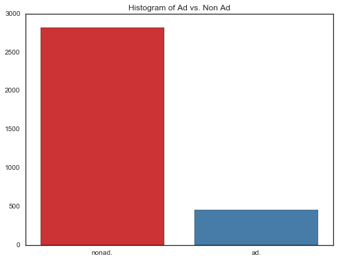
- There are 3,279 rows (2,821 non ads, 458 ads)
- There are 1,558 columns (3 continous; others binary)
- 28% of instances are missing some of the continuous attributes.
- Class Distribution - number of instances per class: 2,821 non ads, 458 ads.
- height, width and aratio are the only continuous variables
Data Cleaning
vars_cont = ['height','width','aratio']
'''
    Clean up 3 continuous variables:
        - Replace ? with NA
        - strip balnks
        - convert to float
'''
dat[vars_cont]= dat[vars_cont].apply(lambda x: x.str.strip()).replace("?",np.nan).astype(np.float)
'''
    Clean up Local - this should be 0,1
        - Replace ? with 2 (unknown can be its own category)
        - Convert instances were there are strings for 0 and 1 to integers
'''
dat['local']= dat['local'].replace("?",2)
dat.loc[dat.local == '1','local'] = dat[dat.local == '1'].local.astype(np.int64)
dat.loc[dat.local == '0','local'] = dat[dat.local == '0'].local.astype(np.int64)
Data Exploration
In doing some data exploration, we can see that there are indeed more Non-Ads than Ads, and that some of the continuous variables need to be scaled.
# Plot Ad vs Non Ad histogram
fig, ax = plt.subplots(ncols=1, nrows=1, figsize = (8,6));
data = dat.target.value_counts()
data= data.reset_index()

sns.barplot(data=data, y= 'target', x='index', palette='Set1', ax =ax);
labels = [item.get_text() for item in ax.get_xticklabels()]
ax.set_xticklabels(labels, rotation = 0)
ax.set_title('Histogram of Ad vs. Non Ad')
ax.set_xlabel('')
ax.set_ylabel('')
plt.show(fig)
'''
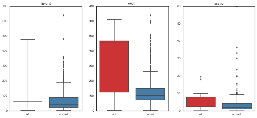
    Box plots of continuous variables vs target
        - Need to scale height & width since these are not on the same scale
'''
var = ['height','width', 'aratio']
fig, axes = plt.subplots(figsize=(14, 6),ncols=3)
for i, v in enumerate(var):
    sns.boxplot(x = 'target', y =v, ax = axes[i], data=dat[[v, 'target']], palette='Set1')
    axes[i].set_xlabel('')
    axes[i].set_ylabel('')
    axes[i].set_title(v)
plt.show(fig)
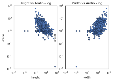
Plotting the continuous variables on a log scale enables us to see that there are linear relationships between the variables and outliers that we can remove.
'''        As Height increases, Aratio decreases - negative correlation expected
        As Width increases, Aratio increases - positive correlation expected
'''
fig, axes = plt.subplots(figsize=(6, 4), ncols=2)
dat.plot.scatter(x = var[0], y = var[2],ax=axes[0], title = 'Height vs Aratio - log', loglog = True)
dat.plot.scatter(x = var[1], y = var[2],ax=axes[1], title = 'Width vs Aratio - log', loglog = True)
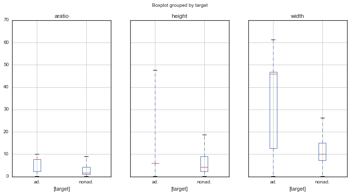
After scaling continuous features and removing outliers:
Correlation
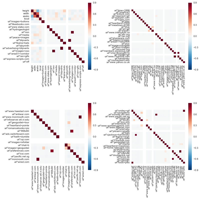
After doing some exploratory analysis, it looks like some of the features are correlated with one another, and there is some correlation among the three continuous variables.
corrmat = dat.corr()
# first 100 features - how correlated are they?
# There are quite a few highly correlated features in the data
corr_1 = corrmat.iloc[0:20,0:20]
corr_2 = corrmat.iloc[21:50,21:50]
corr_3 = corrmat.iloc[51:70,51:70]
corr_4 = corrmat.iloc[71:100,71:100]
# plot correlations of 1st 100 features to gain insight
# plot correlation matrix
fig, axes = plt.subplots(figsize=(12, 12), nrows=2, ncols=2)
fig.subplots_adjust(hspace=.5, wspace=.5)
sns.heatmap(corr_1, vmax=.9, square=True, ax=axes[0][0]);
sns.heatmap(corr_2, vmax=.9, square=True, ax=axes[0][1]);
sns.heatmap(corr_3, vmax=.9, square=True, ax=axes[1][0]);
sns.heatmap(corr_4, vmax=.9, square=True, ax=axes[1][1]);
Exploratory Summary
After doing some exploratory analysis, it is clear that there is are more Non-Ads than Ads in the dataset (84% vs 16%). There are many features in the data, and it looks like a lot of them have majority value equal to 0, so I think that these may not add much information to the data.
Also, there are many features that are highly correlated in the dataset. Since there are so many features in the data, next I will explore PCA to reduce dimensionality and penalized logistic regression. As a last step, I want to also explore random forests since they have embedded feature importance based on Gini impurity/ information gain.
PCA and Logistic Regression
Principal Components Analysis (PCA) is a technique that is often used to reduce the numbers of features in a dataset with highly correlated features to a smaller number of principal components which explain most of the variance of the observed variables.
'''
    Use PCA to reduce dimensionality and then run logistic regression
'''
# use PCA to reduce dimensionality
pca = decomposition.PCA()

# use logistic regression to predict target
logreg = LogisticRegression()

# build pipeline to combine PCA and Logistic Regression
pipe = Pipeline(steps=[('pca', pca), ('logistic', logreg)])

# n_components for PCA - for gridsearch
n_components = [100, 140, 160, 180]

# logistic regression - for gridsearch
Cs = np.logspace(-4, 4, 3)

# parameters for logistic regression and PCA
params_grid = {
    'logistic__C': Cs,
    'pca__n_components': n_components,
}

# estimator does gridsearch for best n_components and best C value
estimator = GridSearchCV(estimator=pipe, param_grid=params_grid)

# fit estimator
estimator.fit(X_train, y_train)

# run estimator on test set and get predictions
predictions = estimator.predict(X_test)
Classification Report:
| Class | Precision | Recall | F1-Score |
|---|---|---|---|
| Ad | 0.96 | 0.71 | 0.82 |
| Non-Ad | 0.95 | 0.99 | 0.97 |
| avg/total | 0.95 | 0.95 | 0.95 |
Confustion Matrix:
| Ad_Predicted | Non-AD_Predicted | |
|---|---|---|
| Ad_Actual | 25 | 10 |
| Non-AD_Actual | 1 | 199 |
PCA and Logistic Regression Results discussion
While running PCA and Logistic Regression using gridsearch for finding the best parameters took a bit of time, the results are pretty good. Running PCA reduces the dimensinality of the data to 160 features which is not surprising given the exploratory analysis which showed many highly correlated features and features with practically all 0’s.
Using 90% of the data for training and 10% for testing, the model has a score of 95%. The classification report indicates that the model makes errors when it predicts Ads as Non-Ads, which reduces the recall and F1 scores.
Next, I am interested in running Logistic Regression using L1 penalty to reduce the coefficients to zero for feature selection.
Logistic Regression using L1 penalty
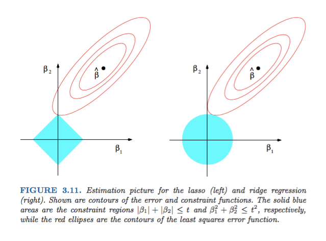
Regularized Logistic Regression is a technique used for classification problems when there are many features in the data. L1 regularized logistic regression can be used for feature selection because it has the property that it can push feature coefficients to 0. Mathematically, this is due to the L1 norm penalty constraint that it imposes on the function.
When compared to Ridge Regression which used L2 penalty, we can see that graphically from ESL (Hastie, Tibshirani, Friedman):
'''
    Logistic Regression using L1 penalty which automatically does feature selection
'''

X_train, X_test, y_train, y_test = train_test_split(X, y, test_size=0.10, random_state=2)

params_grid_1 = {'C': Cs,}
# use L1 penalty
logreg_L1 = LogisticRegression(penalty='l1')
# perform grid search for best C value
estimator_L1 = GridSearchCV(estimator=logreg_L1, param_grid=params_grid_1)
# train model
estimator_L1.fit(X_train, y_train)
# print score on training set
print estimator_L1.best_params_, estimator_L1.best_score_
# run L1 Logistic Regression estimator on test set and get predictions
predictions_L1 = estimator_L1.predict(X_test)
Classification Report:
| Class | Precision | Recall | F1-Score |
|---|---|---|---|
| Ad | 1.00 | 0.88 | 0.93 |
| Non-Ad | 0.97 | 1.00 | 0.99 |
| avg/total | 0.98 | 0.98 | 0.98 |
Confustion Matrix:
| Ad_Predicted | Non-AD_Predicted | |
|---|---|---|
| Ad_Actual | 35 | 5 |
| Non-AD_Actual | 0 | 195 |
Logistic Regression using L1 penalty Results discussion
The score for logistic regression using L1 penalty is close to 98%, so it is better than that of PCA + Logistic Regression. Also, the above model misses fewer times when predicting an Ad as a Non-Ad, and thus has a higer F1 score.
The model does feature selection by shrinking coefficients down to 0 for features that dont explain the data well. When looking at the features with highest coefficients sorted in decreasing order, we can see that ‘ancurl news’ is at the top along with ‘alt information’.
Lasty, I want to explore feature importance using a Random Forest Classifier in order to compare features importances and scores.
'''
FEATURE IMPORTANCE USING Random Forest Classifier
'''
# split data into training and test sets
X_train, X_test, y_train, y_test = cross_validation.train_test_split(X, y, test_size=0.10, random_state=3)

# Random Forest Classifer
rf = RandomForestClassifier(n_estimators = 1500)
rf.fit(X_train, y_train)
print "Random Forest classifier score on training set", rf.score(X_train, y_train)
rf_predicted = rf.predict(X_test)
print "Random Forest classifier score on test set", rf.score(X_test, y_test)
Classification Report:
| Class | Precision | Recall | F1-Score |
|---|---|---|---|
| Ad | 0.97 | 0.83 | 0.90 |
| Non-Ad | 0.97 | 0.99 | 0.98 |
| avg/total | 0.97 | 0.97 | 0.97 |
Confustion Matrix:
| Ad_Predicted | Non-AD_Predicted | |
|---|---|---|
| Ad_Actual | 30 | 6 |
| Non-AD_Actual | 1 | 198 |
Random Forest Classifier Results discussion
The performance of the Random Forest Classifier is not as good as that of Logistic Resgression using L1 penalty (98% vs. 97%) but it is very close to that of PCA + Logistic Regression. The top features (based on importance) are not the same as those with the highest coefficients which makes sense given that one is optimizing based on feature impurity while the other is not.
Final thoughts
In conclusion, I went through a few algorithms to predict if an image will be an advertisement or not based on its attributes, and all of these predicted with over 90% accuracy on the test set. If I had to chose, I would implement Logistic Regression with L1 penalty because it scored the highest and reduced the dimensionality in the dataset which is important when dealing with so many features. However, I also think the Random Forest model also performed very well and did not need much tuning, so it could also be implemented.